A structured guide helps beginners understand how a NeRF model learns a 3D scene from a group of 2D images. A NeRF system studies how light behaves, how density changes across space, and how colors appear from different viewing directions. A clear explanation of data preparation, ray creation, positional encoding, model structure, and rendering makes the training workflow easier to follow. A simple approach ensures that even new learners can train a NeRF model using PyTorch.
Table of Contents
Understanding the Needs of a NeRF Model
A NeRF works by learning a continuous function that converts coordinates and view directions into density and color.
The training process needs:
- Input images of the same scene from different angles
- Camera pose information for every image
- A neural network built with PyTorch
- A renderer based on volumetric rendering
The model learns depth, geometry, and appearance through repeated comparisons with real image pixels.
Preparing the Dataset
A well-structured dataset is important for accurate training.
Each scene normally includes images and a file containing camera intrinsics and extrinsics.
Dataset Structure
| Component | Description |
|---|---|
| Images | Multiple RGB images captured from different viewpoints |
| Camera Intrinsics | Focal length, resolution, and optical center values |
| Camera Extrinsics | Camera positions and rotations for every image |
| Transforms File | The JSON file storing all camera parameters for training |
Synthetic datasets usually come from Blender, while real-world datasets follow LLFF-style formats.
Installing Required Libraries
A basic NeRF training environment requires a few Python libraries:
- PyTorch
- NumPy
- ImageIO
- tqdm
- Matplotlib
Building the NeRF Network in PyTorch
A NeRF model uses a multi-layer perceptron (MLP) to map encoded spatial coordinates into color and density.
Important features include:
- Positional encoding to capture detail
- Skip connections for stability
- Separate outputs for color and density
NeRF Architecture
| Layer | Description |
|---|---|
| Input Layer | Receives encoded xyz coordinates and viewing directions |
| Hidden Layers | Stacked linear layers with ReLU activation |
| Skip Connections | Adds original inputs to deeper layers to improve precision |
| Sigma Output Head | Predicts density at each sampled point |
| Color Output Head | Predicts RGB values influenced by direction and density |
Understanding Positional Encoding
Positional encoding converts low-frequency coordinate values into rich features using sine and cosine functions.
The transformation helps NeRF capture:
- Fine details
- Sharp edges
- Small textures
- High-frequency lighting
Encoded inputs allow the MLP to represent complex patterns more easily.
Generating Rays From the Camera
Every pixel in an input image becomes a ray entering the 3D scene.
Ray generation uses camera intrinsics and camera pose.
Ray Components
| Component | Explanation |
|---|---|
| Ray Origin | The camera’s position in 3D space |
| Ray Direction | The normalized direction of the pixel’s viewing vector |
| Near/Far Bounds | Minimum and maximum depths for ray sampling |
| Samples per Ray | Number of depth points tested along each ray |
Well-generated rays produce more accurate scene reconstruction.
Sampling Points Along Rays
The NeRF renderer samples points at different depths.
At each point:
- Positional encoding is applied
- The neural network predicts density and color
- The renderer stores these predictions for final blending
Common values include:
- 64 samples for coarse prediction
- 128 samples for fine prediction
These samples help the system understand both global shapes and tiny surface details.
Applying the Volume Rendering Equation
Volumetric rendering blends density and color predictions to produce a final pixel value.
The process simulates how light accumulates and fades as it travels through space.
The equation considers:
- Color contribution from each sample
- Absorption based on density
- Transparency of the medium
- Distance between sample points
This method creates soft shadows, highlights, and smooth transitions.
Defining the Loss Function
A NeRF model learns by comparing its rendered pixels with real image pixels.
Useful losses include:
- Mean Squared Error (MSE)
- PSNR for monitoring training quality
The training loop reduces the error over time, improving the scene’s accuracy.
Training with the PyTorch Loop
The training loop drives the learning process.
Each iteration includes:
- Selecting a random image
- Choosing random pixels
- Creating rays
- Sampling from the scene
- Predicting density and color
- Rendering the final pixel
- Calculating loss
- Backpropagating gradients
- Updating model weights
Training Loop
| Step | Function |
|---|---|
| Batch Selection | Picks a subset of pixels from images |
| Ray Marching | Samples 3D points along selected rays |
| Forward Pass | Predicts density and RGB using the NeRF model |
| Volume Rendering | Blends sample information into pixel colors |
| Loss Calculation | Compares predicted pixels with actual ones |
| Backward Pass | Computes gradients using backpropagation |
| Weight Update | Adjusts parameters with the optimizer |
Saving and Testing the Model
A trained NeRF can render new viewpoints not present in the original dataset.
Evaluation involves:
- Rendering a 360° path
- Generating depth maps
- Saving model weights
- Creating videos or detailed still images
High-quality results show accurate geometry and realistic lighting.
Tips for Better NeRF Training
Training quality improves with:
- Larger image sets
- Clean and consistent camera calibration
- Higher resolution input images
- More samples per ray
- GPU acceleration for faster training
Advanced techniques such as hash-grid encoding and importance sampling greatly speed up NeRF training for large scenes.
Closing Reflections
A clear step-by-step workflow helps beginners understand how to train a NeRF model using PyTorch. A simplified explanation of data preparation, ray creation, positional encoding, model prediction, and volumetric rendering builds confidence for new learners. A practical and structured approach supports the creation of detailed and realistic 3D reconstructions from ordinary photographs.